Using VLOOKUP() function in Excel

VLOOKUP() function is very useful when you want to update a column values by taking some reference from another sheet or same sheet column values.

Here i have two sample sheet first sheet is "Student" in which we have three columns (student name, Grade, Marks) and second sheet is "Grade" in which we have two columns (Grade, marks) as showing in following images.

Sample Sheet01 "Student" :

Sample Sheet02 "Grade" :

Now our objective is to update the column "Marks" of "Student" sheet by referring "Grade" column of second sheet "Grade" using VLOOKUP() function. Following are the steps to update column "Marks" using VLOOKUP() :

• Select first cell (C2) of marks in  "Student" sheet and hit on formula tab and click on 'Lookup & Reference' and then hit on VLOOKUP as highlighted in below image.

•  A lookup window will pop-up as showing below image. Select whole column "B" (Grade) to provide the value in "Lookup_value"  .

• 
  

• To give the value in "Table_Array" select second sheet and select both the column "Grade" and "Marks"  and give "Col_index_num" = 2 as 'Marks' is in the second column which need to be refer and for "Range_lookup" give as "False" as showing in below image.     

   

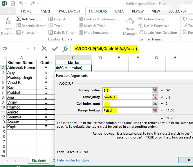
•  Once you complete above steps hit on "OK" button and you can see a complete vlookup formula as =VLOOKUP(B:B,Grade!A:B,2,FALSE) . which will update the cell "C2" with respective marks. Drag and drop it till end to update all the values.